Radiation measurement

With respect to the actual monitoring purpose the relevant sources of ionizing radiation are substances which are subject to spontaneous decay. This is the case with isotopes with instable atomic nuclei as opposed to their stable variants. Spontaneously their nuclei split into smaller nuclei (mostly unstable as well). The decay goes along with the emission of particles—Helium nuclei (alpha radiation) or electrons (beta radiation)—and/or energy quanta (gamma radiation).

Radiation detectors

Ionizing radiation can be detected by utilizing its ionizing effects. Best known, and widely applied, is the Geiger-Müller counter tube: A hermetically closed glass cylinder is filled with a noble gas (Argon or Xenon). The inner surface of the cylinder is coated with an electrically conductive layer. A thin metallic wire is mounted, isolated from the coating, in the middle axis of the cylinder. The wire and the conducting coating will be used as electrodes. An atom of the gas filling, that will be hit by a particle or quantum irradiated by radioactive materials in the ambience, will be ionized, i.e. the gas atom will be split into a positive ion and an electron. Let us assume that we apply a high voltage of e.g. 500V DC between the electrodes. Due to the electrical field between the electrodes the electrons will move towards the positive electrode while the (positive) ions will move towards the negative electrode where they will recombine with electrons. For every split and recombined atom one electron has to pass the outside circuit thus generating an elementary current impulse.

Other detection mechanisms utilize ionizing effects in the semiconductor layers of PIN diodes, or they make use of scintillators. In a scintillator crystal high-energy quanta are converted into avalanches of photons which are captured by a photo detector (e.g. a photo diode).

Technical realisation

The frequency of events which cause electrical impulses can be taken as a measure for the intensity rate of radiation emitted in the abbience of the detector. Hence the task is to count, within an appropriate time interval, the impulses generated by the detector (which explains the term “counter tube”). The choice of the time interval depends on the purpose of the measuring task since the generation of impulses is subject to a stochastic process, i.e. a case of likelihood.

Radiation levels are stochastic quantities

The likelihood of the event of an eventual impulse depends on several processes. The likelihood chain starts with the random decay of an atom of the radioactive isotope. The released particle or quantum resp will pass the detector space only accidentally since it could be ‘shot’ into any spacial direction. Finally, not every particle or quantum passing the detector space will cause an interaction which results in an electrical impulse. All those probabilities are to be multiplied thus leading to a random number of events counted within a given time interval even at a constant exposure rate.

The distribution of counter results is described by means of a probability-density function. The Poisson distribution underlying this type of random process can be approximated by the well-known Gaussian distribution. Its maximum represents the mean value of a large number of counter results at constant exposure rate. The segments of the area below the curve represent the number of results falling into the respective segment.

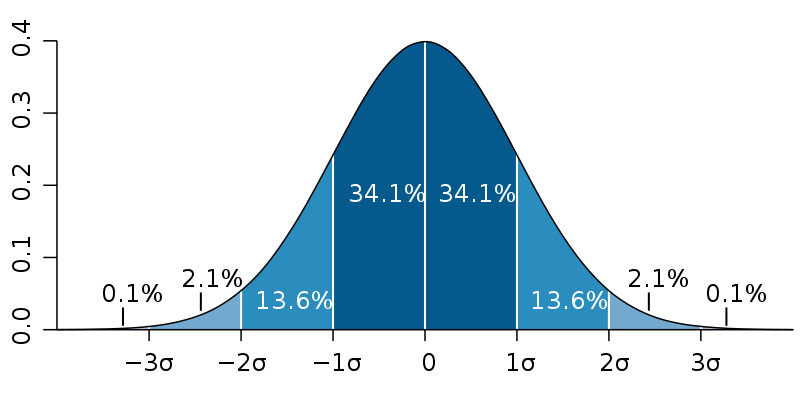Probability-density function (source: M.W.Toews, Quelle: Wikipedia)

A Gaussian distribution is characterized by its maximum (aka ‘expectation’) and the standard deviation σ represented, in above figure, by the (equal) width of segments. Due to the underlying Poisson distribution the standard deviation is given, in the actual case, by the square root of the expectation. Let us give a numerical example:

• Let the mean number of events counted within an interval of 15 minutes be 100 (which approximates the conditions implemented by the TDRM sensor stations).
• The standard deviation σ then would be 10 counts or 10% of the mean value.
• Hence two thirds of results would lie within the interval from 90 to 110, another third would lie outside of the ±10% range.
• A narrowing of the standard deviation range to ±1% would require an extension of the counter interval by a factor of 100 (!), hence 25 hours.
• The standard deviation range would shrink also with increasing intensity of radiation. An (abnormal) increase by a factor of 10 would result in a decrease of the standard deviation range to ±3%.

The numerical example illustrates the inevitable trade-off between sensitivity and response time associated with the measurement of stochastic phenomena.

We decided to set the counter interval to 15 minutes in favor of a fast response. With respect to the purpose of the monitoring network we take it for most important to indicate irregular situations without delay rather than to resolve it to the finest degree. Every minute a TDRM sensor stations delivers the result of events counted within a ‘sliding window’ of the past 15 minutes. Hence trends can already be estimated after a couple of minutes.

Typical time diagram of measurements: variations of the radiation level are of stochastic origin rather than fluctuations of the dose rate of the ambient atmosphere